scRNA sequencing (scRNA-seq) is a common and powerful technique for profiling the whole
transcriptome of a large number of individual cells. The analysis of the huge volumes of data
generated by these experiments requires the use of sophisticated statistical and computational
tools. In RNA sequencing, RNA is typically extracted from a tissue that contains a variety of cell
types. This issue has been solved by using a single cell. Cells would be sorted prior to RNA-seq,
and RNAseq would be performed on specific cell types separately. The data will then be
analyzed using a variety of cell types.
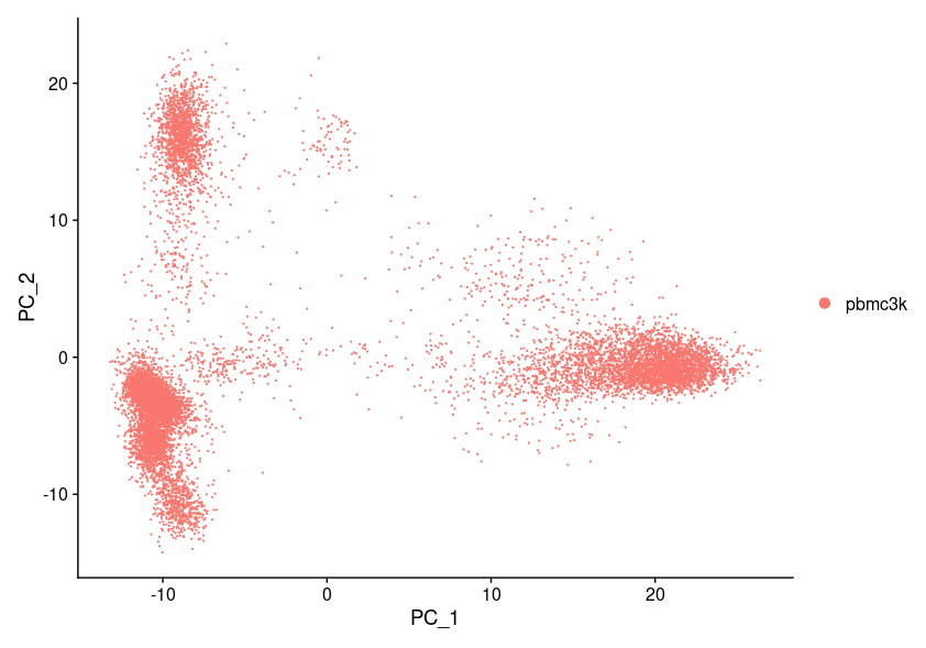
Figure #1: scRNA PCA
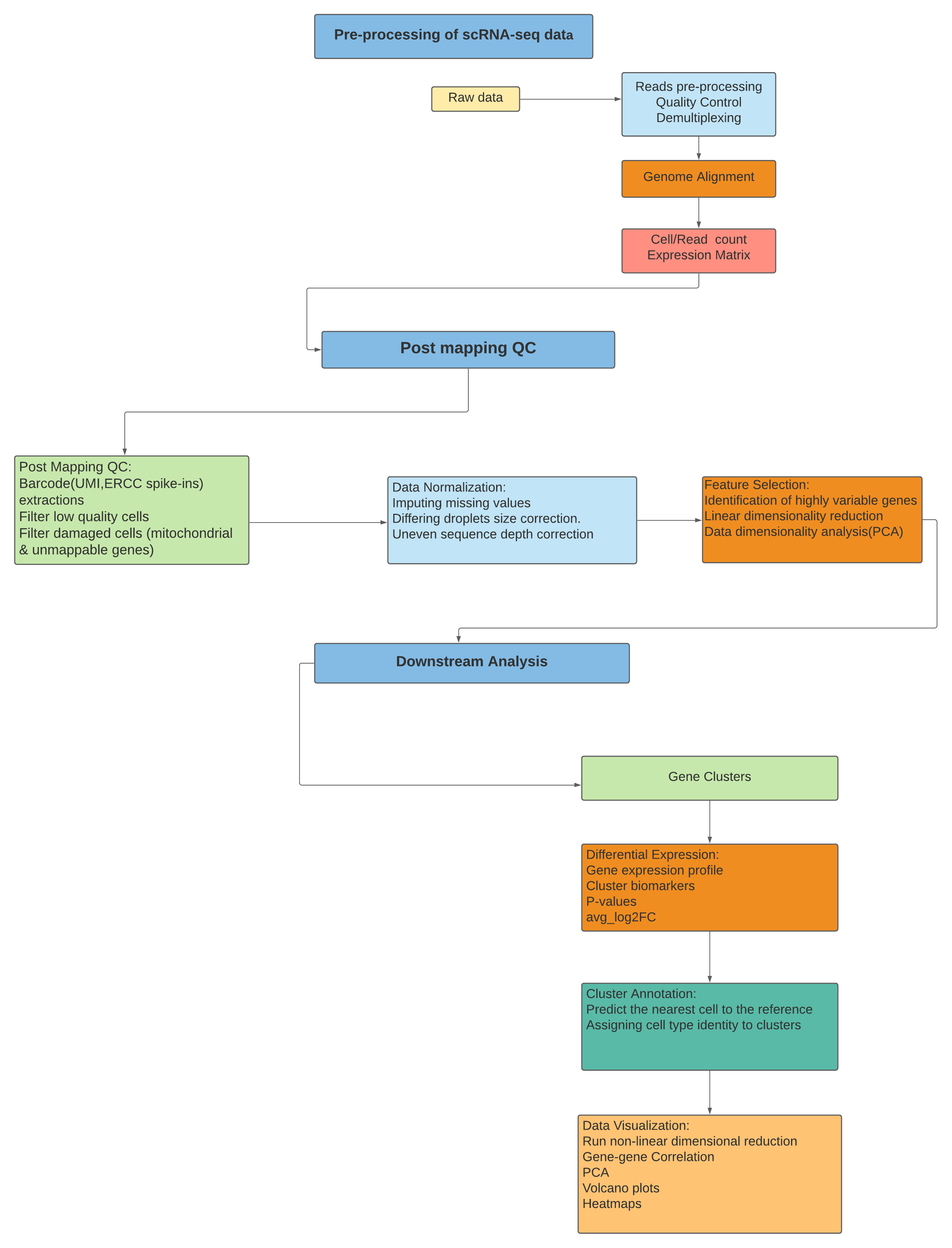
Three Main Stages for Performing scRNA-Seq Data Analysis
scRNA-Seq is processed for the first part like general steps for any high throughput sequencing
data. However, after mapping and read count, the later steps require a mix of existing RNASeq
analysis methods and novel methods to address the technical difference of scRNASeq. Finally,
the biological interpretation is analyzed with methods specifically developed for scRNASeq.
Followed is the workflow we use to perform scRNA-seq analysis.
Regardless of droplet method, the following are important for a good quantification at the cellular level
Sample Index: to keep track of which sample the read come from
Cellular barcode: to keep track of which cell the read come from
Unique molecular identifier (UMI): to find out of which transcript molecule the read comes from
Sequencing read1: the read1 sequence
Sequencing read2: the read2 sequence
In RNA sequencing, RNA is typically extracted from a tissue that contains a variety of cell types.
This issue has been solved by using a single cell. Cells would be sorted prior to RNA-seq, and
RNA-seq would be performed on specific cell types separately. The data will then be analyzed
using a variety of cell types. The following is the workflow we use to perform scRNA-seq analysis:
Step 1 - Quality Control and Data Preprocessing
Formatting reads and filtering noisy cellular barcodes
Assigning reads to their cellular barcodes and molecules of origin
Demultiplexing the samples
Generate a file of counts for each cellular barcode
Step 2 - Mapping
Mapping/pseudo-mapping to transcriptome
Gene assignment
Barcode counts
Step 3 - Post-QC Mapping
Removal of unwanted cells
Unique feature counts
Step 4 - Matrix generation
Collapsing UMIs and Quantification of Reads
Find which cDNA was the origin of the tag a UMI was attached to
Count unique UMIs for (gene, UMI) pairings
Step 5 - Data Normalization
Correct for differing droplets sizes
Impute missing values
Reduce noise, make it easier to identify the structure of the data
Step 6 - Feature Selection
Calculate Cell-to-cell variation in the dataset (i.e., genes that are highly expressed in some cells and lowly expressed in others)
Identify most highly variable gene
Step 7 - Dimensionality Reduction
Perform linear dimensional reduction
Perform PCA analysis
Step 8 - cell Clustering
Gene cluster with their assigned p-values, foldchange ratios, p-value adjustments
Step 9 - Differential Expression for Expressed Features
Find markers for differential expression
Compare distribution of expression levels
Compare values for each gene
Comparison of cell from different replicates
Step 10 - Marker Identification
Find markers for each cluster
Find all markers distinguishing one cluster from another
Find markers for every cluster compared to all remaining cells
Step 11 - Data visualization
Plot variable features
Visualize both cells and features based on their PCA score
Visualize marker expression based on raw counts or differential expression
At USU’s high-performance computing and bioinformatics facility, we have developed a series of parallel, multicore, CPU-based,
open-source pipelines for large-scale -omics data analysis, which enables efficient and parallel analysis of multiple datasets
in a short period of time.